Topic Modelling is a machine learning task. It aims to identify main themes, or subjects, in a corpus of documents. Its uses in healthcare include classifying PubMed entries, extracting diagnoses from clinical notes and generating keywords from a collection of hospital policy documents.
The underlying intuition behind topic modelling is that a corpus of documents contains, explicitly, words; and, implicitly, topics as expressed by these words. Words associated with a given topic will tend to cluster together in documents on that topic. By studying the relationships between words and documents, we can ‘discover’ the topics a priori.
There are three main approaches to modelling topics in documents. The first two, Latent Semantic Analysis (LSA) and Latent Dirichlet Allocation (LDA) take a ‘bag-of-words’ approach, and the last is a language model-based approach (Bertopic).
We’ll cover LDA and BERTopic in subsequent posts. This post takes a quick look at LSA and its cousins Non-negative Matrix Factorization (NMF) and Probabilistic LSA (pLSA).
LSA-Based Topic Modelling
LSA is essentially an application of Singular Value Decomposition (SVD) to a corpus of documents. SVD is a matrix factorization operation that relies on a general property of matrices: that any m x n matrix A can be factorized (‘decomposed’) as follows:
A = U ∑ VT
where
U is m x m (the columns of which are the left singular vectors),
∑ is a diagonal m x n matrix (the singular value matrix), and
VT is n x n (the columns of which are the right singular vectors – remember this is a transpose. U and V are orthogonal).
The math behind SVD is rather complicated (involving eigenvalues and eigenvectors) and I refer you to this article. We won’t need to compute these, since both numpy and scikit-learn have ready-made functions to do this for us. The outputs we’re really interested in are the diagonals of ∑ (the singular values, which are the square roots of the eigenvalues of AAT and are usually denoted as sigma (σ)). The sigma values lie in a different, latent, space from the components of the dataset. The value of a given sigma reflects its contribution to variance in the dataset, and in the decomposition, sigma values are automagically arranged from highest to lowest ie σ1 > σ2 > … σm.
Let’s walk through a toy example of LSA. I have this really small corpus of five documents as follows:-
docs = [ “ball game player score team”,
“cook recipe taste food eat”,
“code computer software program data”,
“team player win ball coach”,
“eat delicious cook meal taste” ]
It might be obvious to you what topics these sentences are about, but that isn’t true of someone who, or some machine that, doesn’t understand English. To discover these topics a priori using LSA, the steps are as follows:
- Construct a Document-Term Matrix (DTM).
- Perform SVD on the DTM.
- Reduce the dimensions of ∑ to k latent topics (optional, but usually done).
- Interpret the discovered topics.
- Associate topics with documents.
The Jupyter notebook for this short exercise can be found in my GitHub if you want to delve into the code.
Our A matrix for LSA is the DTM, where the rows are the docs above, and the columns are the individual words in the vocabulary of the corpus. The matrix entries are the count of occurrences of words in each document.
After decomposing A, we get:
U, which contains the docs (in 5 rows), with each column representing a document-topic association, simplistically speaking.
∑, as explained above. The sigmas represent the ‘strength’ or ‘importance’ of the interaction between documents and topics (U) and topics and words (VT). ∑ is an interesting construct. Its original dimensions correspond to the original dataset, ie 5 x 19 in our corpus. The maximum number of topics (k) that we can discover is min(5,19) = 5 topics. This may sound rather restrictive, but in real life, corpora are much larger than 5 documents, and usually the number of topics we’re going to be interested in will typically be much smaller than the number of documents.
VT(transpose of the right singular vectors) contain the movies (in 19 rows) with each column representing a word and each row representing a topic-word association, simplistically speaking.
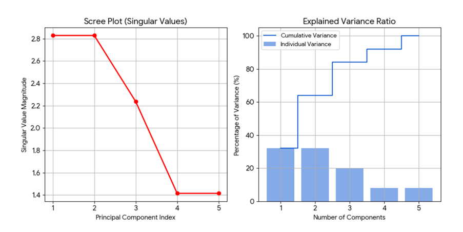
Once we get our ∑ , we reduce its size to the k-number of topics we’re interested in. How do we determine k, other than the min(m,n) restriction? It depends on your appetite for data. But a general rule of thumb is to find the ‘elbow’ by plotting a scree plot to show where a dramatic drop in sigma values might occur. In our dataset, the sigmas found are: [2.82842712 2.82842712 2.23606798 1.41421356 1.41421356] (refer to the Jupyter notebook for details). We then obtain these plots which show the elbow at k=3.
We can then extract and interpret the topics, as follows:-
==============================================
DISCOVERED LATENT TOPICS
==============================================
Topic 1:
 Top Terms: ['taste', 'eat', 'cook', 'delicious', 'meal']
 Weights:   ['0.500', '0.500', '0.500', '0.250', '0.250']
Topic 2:
 Top Terms: ['ball', 'player', 'team', 'coach', 'win']
 Weights:   ['0.500', '0.500', '0.500', '0.250', '0.250']
Topic 3:
 Top Terms: ['software', 'code', 'computer', 'program', 'data']
 Weights:   ['0.447', '0.447', '0.447', '0.447', '0.447']
And finally, associate topics with documents:
==============================================
DOCUMENT-TOPIC ASSOCIATIONS
==============================================
Doc 1 : ball game player score team
  Topic scores: T1=0.000, T2=2.000, T3=0.000
  → Dominant: Topic 2
Doc 2 : cook recipe taste food eat
  Topic scores: T1=2.000, T2=0.000, T3=0.000
  → Dominant: Topic 1
Doc 3 : code computer software program data
  Topic scores: T1=0.000, T2=0.000, T3=2.236
  → Dominant: Topic 3
Doc 4 : team player win ball coach
  Topic scores: T1=0.000, T2=2.000, T3=0.000
  → Dominant: Topic 2
Doc 5 : eat delicious cook meal taste
  Topic scores: T1=2.000, T2=0.000, T3=0.000
  → Dominant: Topic 1
This example is rather contrived, the topics were easily separable. But LSA doesn’t perform well on PubMed abstracts. Possible reasons include syntactic blindness (ignoring negations and word order) and inability to handle polysemy.
Non-negative Factorization
NMF also decomposes a DTM, but into 2 matrices, with the constraint that both these contain only non-negative numbers. Conceptually:
V (m x n) ≈ W (m x k) x H (k x n)
m words x n docs topics-words docs-topics
for k topics.
After random initialization, minimize reconstruction error for W and H iteratively until convergence. The top words for each topic is found in each column of W, and rows of H shows the strength of topics in documents.
Probabilistic LSA
pLSA models the joint probability of a document d and a word w given a topic z, for k topics. It uses the expectation maximization algorithm to find the best P(w|z) and P(z|d). It has largely been replaced by Latent Dirichlet Allocation because it doesn’t generalize well to unseen data, and must be retrained if there are new documents – ie it can’t be used for inference.
Closing Thoughts
This has been a short walk-through of early topic modelling techniques. I spent some time on SVD because I find the concept of an emergent latent space rather intriguing. SVD has other applications that you might find useful in healthcare, such as gene expression analysis, functional MRI analysis, dimensionality reduction and recommendation engines. Nonetheless, LSA, NMF and pLSA have been largely superseded by more recent techniques.
Leave a Reply