Topic Modelling 2: Latent Dirichlet Allocation

Latent Dirichlet Allocation (LDA) is a probability-based topic modelling approach that treats documents as bags-of-words. Conceptually it is similar to Latent Semantic Analysis (LSA, discussed in the previous post) in that it tries to discover a latent space from observed variables, but instead of a deterministic matrix factorization, it uses probability distributions on random variables. Downstream applications of LDA include information retrieval (eg retrieving PubMed abstracts relevant to keywords entered) and classifying documents.

In LDA, we look at two probability distributions:

1. A topic is a probability distribution over words in a vocabulary.
2. A document is a probability distribution over topics.

LDA is performed in two steps: (1) constructing the model, and (2) inference using Gibbs sampling, based on the hyperparameters α and β. A hyperparameter in machine learning is a parameter that controls the learning process or structure of a model, but is not learnt from the data itself. You ‘tune’ it based on your domain knowledge, and various versions of trial-and-error (formally: grid search, random search, Bayesian search etc….).

Model Construction

Our starting point for constructing the model is a corpus of documents.  (LDA only makes sense if you have a corpus of documents to train on; you wouldn’t get a meaningful probability distribution of topics from a single document. You can, of course, use an LDA model to make an inference on a single document.)  The corpus has a vocabulary of words, distributed across the various documents. Our aim is to discover the ‘hidden’ topics among the words, on the assumption that particular words are associated with a given topic. That’s certainly a reasonable assumption, isn’t it?

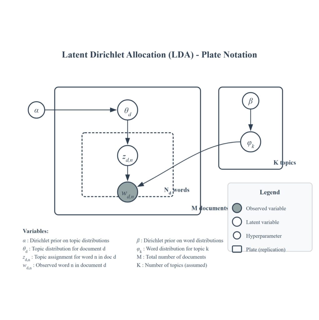
So, we construct a model based on two Dirichlet distributions: topics in M documents (controlled by the hyperparameter α, and words in k topics (controlled by the hyperparameter β). A Dirichlet distribution is a probability distribution over probability distributions. It generates a vector of probabilities that sum to 1, making it useful for modelling proportions (‘what proportion of a document talks about each topic?’). The α hyperparameter (actually a vector of  k topics) controls the shape of the distribution. If you’re familiar with statistics, the dirichlet distribution is just the multi-variate generalization of the beta distribution (not to be confused with the β hyperparameter of LDA, which is really just another α hyperparameter for the second dirichlet distribution given a different name to avoid confusion).

The only observed variable in our model is W_d,n (word n in document d). The rest of the variables (ϑ_d: topic in document d, Z_d,n: topic assigned for word n in document d, ϕ_k:  word distribution for topic k) are latent variables that are discovered during inference (see Gibbs sampling section).   The model is often represented by a plate notation diagram as shown in Figure 1.

Gibbs Sampling

Gibbs Sampling is one type of Markov Chain Monte Carlo that generates a sequence of samples from a multivariate probability distribution. If that sounds like gibberish, the steps can be explained as follows: –

1. We start off with our assumed hyperparameters k, α and β. Say we think there are 3 (k = 3; α = {α₁, α₂, α₃}) topics (Procedure, Diabetes and Clinical Trial) in 5 documents. At the start, the model initializes randomly every word in our 5 documents to Procedure, Diabetes or Clinical Trial.
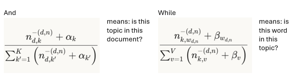
2. For each word in each document – say, the word ‘colonoscopy’ in Document 4 – the model asks:
   • Based on α, does Doc 4 have a lot of Procedure topics?
   • Based on β, do other documents with Procedure use the word ‘colonoscopy’?
3. The model then re-assigns ‘colonoscopy’ to the most likely topic.
4. After many rounds (hundreds or thousands), the words ‘colonoscopy’, ‘polyp’ and ‘biopsy’ will gravitate together because the math of α and β will push them together.

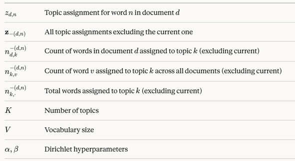
Here’s the math: the probability of topic k, given words in documents, α and β,  is given by the equation

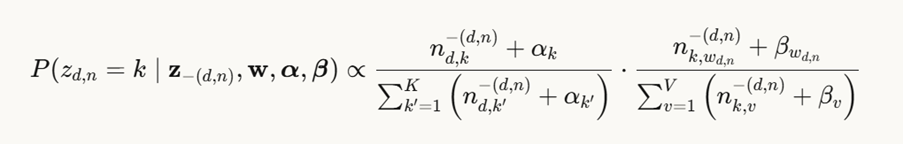
where

Optimal α and β hyperparameters

Clearly the choice of hyperparameters α and β is crucial. How should we ‘tune’ them? Table 1  summarizes the considerations.

		High ( > 1)	= 1	Low ( < 1)
α	Topics per doc	Each document will have many topics	All documents have the same number of topics	Each document focuses on a few topics
β	Word per topic	Each topic has a wide variety of many different words	All topics have the same number of words	Topics will be composed of a few specific key words

If all this is too much for you, I highly recommend you watch these two videos, which are the best that I’ve found when researching this topic, and explain it much better than I can.

Hands On

For our hands-on exercise, we’ll try to extract topics from PubMed abstracts. The Jupyter notebook for this (PubMed_LDA_5K.ipynb) can be found at my GitHub if you want to dig into the code. In case you have issues with the pyLDAvis visualization with the notebook, there is also a html version of a completed notebook where you can see the pyLDAvis visualization, but can’t interact with it. But before we begin, let’s think a bit about what our α and β should be for scholarly journal articles. Essentially, we’re asking ourselves, generally speaking:

1. How many topics would a PubMed abstract contain?  It is usually not one or two, typically there is a blend of several topics being discussed – maybe surgery, nutrition and oncology in the same article. So we should tune our α a bit higher.
2. How many words would a topic be likely to consist of? Here our domain knowledge tells us that medical jargon tends to be specific for a given topic, so we’ll choose our β to be lower.

But in fact, people have done this research for us already (1,2), and have come up with rules of thumb. For shorter documents like abstracts, lower α encourage sparser topic distributions, while full text documents may benefit from slightly higher values. Also, α tuning has more pronounced effect than β tuning on model quality. A rule of thumb is to set β at 0.01-0.1 while α is set at 50/k.

Our hands-on exercise uses gensim’s LdaModel method, where we can specify k, α and β in the parameters num_topics, alpha and eta respectively. Here’s the API reference for gensim. Since α and β are vectors, gensim allows you to specify a list for both. You can even specify a string – ‘symmetric’, ‘asymmetric’ or ‘auto’. ‘Symmetric’ just means all the α values in the vector are the same. We use ‘auto’ here as this allows auto-tuning of the hyperparameter during inference. Gensim doesn’t explain how, but it is likely by Bayesian optimization.

Evaluation

The metric for evaluating LDA performance is coherence, which measures how interpretable and semantically meaningful the topics discovered are to humans by assessing the degree to which high-scoring words within a discovered topic are related to each other. Coherence is derived through a pipeline of 4 steps: segmentation, probability estimation, confirmation measure and aggregation.

1. Segmentation – the top N words for a given topic are segmented into sets, according to the metric’s segmentation strategy (eg all pairwise combinations of the top N words).
2. Probability estimation – the co-occurrence probabilities between word segments are calculated based on a reference corpus (which can be the corpus itself or an external reference corpus). The calculation method varies according to metric eg co-occurrence in documents.
3. Confirmation measure – this measures how much the co-occurrence or relatedness of words support the idea that they belong to the same topic. Again this is specific to metric used eg logarithmic conditional probabilities.
4. Aggregation – individual confirmation scores for all word segments are then aggregated to produce a single coherence score for that topic, typically by averaging or summing. The overall coherence of the model is averaged to produce an overall coherence.

Coherence tends to increase with the number of topics and with the size of the dataset.

These are some information blogs on topic coherence for further reading:

1. https://towardsdatascience.com/understanding-topic-coherence-measures-4aa41339634c/
2. https://towardsdatascience.com/c%E1%B5%A5-topic-coherence-explained-fc70e2a85227/
3. https://www.baeldung.com/cs/topic-modeling-coherence-score

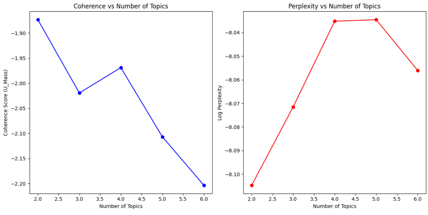
Another metric commonly used in text processing is perplexity. So we can run the model using various values of k, and plot coherence and perplexity scores on a scree plot. We then use the elbow method to pick the k value beyond which coherence plateaus. Figure 2 shows the coherence and perplexity plots for our PubMed sample dataset of 5000 abstracts. It looks like k = 4 is a good bet.

Visualization

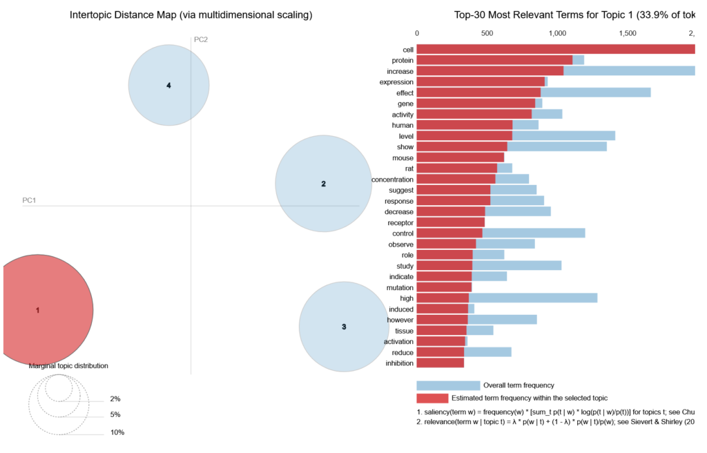
There’s a really nifty visualization tool that integrates nicely with gensim, pyLDAvis, which creates interactive 2-D plots. Figure 3 shows the plot for 4 topics, with Topic 1 highlighted. You can surmise that it is about gene studies. A coherent topic model will have non-overlapping circles scattered evenly throughout the plot.

Closing Thoughts

LDA usually outperforms LSA, at higher computational cost, for a few reasons. Firstly the dirichlet priors α and β encourage sparsity, which reflects our real-world experience of documents typically having a few topics, and topics using only small subsets of vocabulary, whereas LSA assigns some weights to all latent dimensions, and all words contribute to all dimensions, thus making topics ‘fuzzier’.  Secondly, you can tune LDA, whereas you can’t tune LSA. Finally LDA tends to handle polysemy better, simply because it takes a probabilistic approach – words can belong to multiple topics with different probabilities.

Having said that, it seems rather strange that there can only be four topics in a corpus of 5000 PubMed abstracts.  Clearly, LDA is not granular enough for our purpose. In our next post, we’ll look at yet another approach to topic modelling – this time using language models.

References

 1.          Hagg LJ, Merkouris SS, O’Dea GA, Francis LM, Greenwood CJ, Fuller-Tyszkiewicz M, et al. Examining Analytic Practices in Latent Dirichlet Allocation Within Psychological Science: Scoping Review. J Med Internet Res. 2022 Nov 8;24(11):e33166.

2.           Pamungkas Y. Leveraging Topic Modelling to Analyze Biomedical Research Trends from the PubMed Database Using LDA Method. J Sisfokom Sist Inf Dan Komput. 2024 Jun 10;13(2):237–44.