Topic Modeling 3a: BERTopic Part 1

BERTopic is a sophisticated topic modelling technique that combines traditional natural language processing (NLP) and language models (LM). It takes a bit of digging to understand the workings of BERTopic, but I think it is worthwhile because the library seems to be maintained and continues to be updated with integrations to modern LM libraries like LangChain, LlamaCPP and Ollama and platforms like OpenAI and Huggingface.

The official BERTopic site is its GitHub repository maintained by Maarten Grootendorst and located at https://maartengr.github.io/BERTopic/index.html. There is another separate site, www.bertopic.com, that states it is “an independent site providing documentation, guides and links to the official project repositories.”  But all the information you’ll need for starting a BERTopic project can be found at the official site.

In Part 1 of this post, we look at BERTopic’s inner workings.

How BERTopic Works

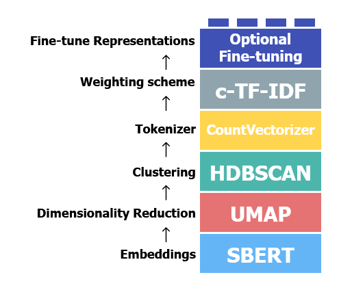
BERTopic is essentially a pipeline comprising 5 required and 1 optional steps, as represented by Figure 1, which also displays the default toolkit used for each processing step. It is modular, such that you can swap out the default tools for each step with those you fancy.

To fully understand how it works and exploit its full potential, you need to know some basics of:

1. LMs -in particular embeddings,
2. Machine learning – in particular dimensionality reduction and clustering,
3. Traditional NLP concepts – in particular tokenization and Term Frequency-Inverse Document Frequency (TFIDF).

You also need to appreciate that although Figure 1 gives the impression that it is a linear process, under the hood there are two parallel tracks going on. Let’s study each of these in some detail as they relate to BERTopic, starting with the first step: embeddings.

Embeddings

Embeddings are numerical representations of text, and early in their history existed simply because neural networks work only with numbers. Since then, they have become useful intermediate data products for several other purposes in NLP. In BERTopic’s case, text is converted to embeddings so that it can be clustered by HDBSCAN (see Figure 1). You generate embeddings with a LM, and that’s all the involvement the LM has in the default pipeline.

To create an embedding from a piece of text, you need a method and a LM. The default method used is Sentence-Transformers, which I highly recommend – it’s practically the de facto standard for creating embeddings. The default LM is quite capable, but for our purpose in our hands-on exercise using PubMed abstracts, I’m replacing it with a model finetuned on PubMed – PubMedBERT Embeddings. This was recommended by Claude Opus 4.6 as “the most practical, plug-and-play…..lightweight” option which integrates seamlessly with sentence-transformers, and is based on Microsoft’s PubMedBERT, which was pretrained on the full PubMed corpus. What better fit can you get for a proof-of-concept exercise?

Dimensionality Reduction

Dimensionality reduction is a family of techniques in machine learning that essentially zip data for machine learning algorithms. In simple terms, reducing dimensions effectively reduces noise in the data up to a point.

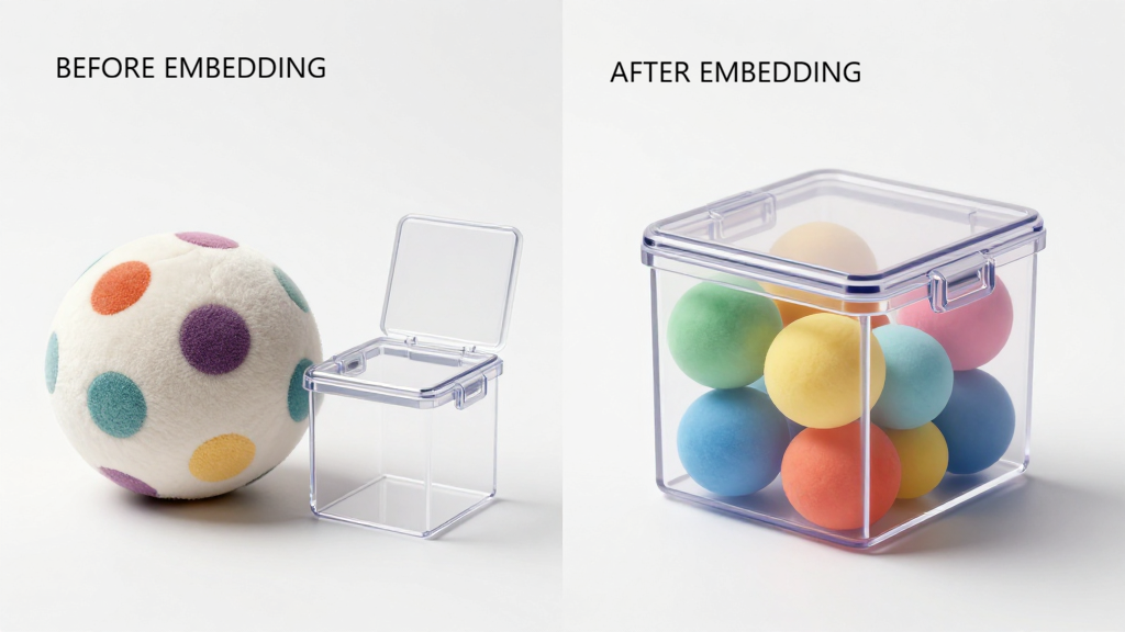
In fact, embeddings are a form of dimensionality reduction themselves. A corpus of documents’ dimension is essentially its entire vocabulary, because each unique word is a dimension. Embeddings shoehorn that vocabulary and the corpus into standard dimensions within a vector space. It is like stuffing a huge, misshapen multi-color plush toy into a tiny square box. The toy is now a very compact cube, and the colors concentrated. (No, that didn’t come from an AI).  In our case, our PubMedBERT Embedding model has 768 dimensions.

In BERTopic, a second dimensionality reduction step is taken to further shrink dimensions as clustering models (used in the next step) tend to handle high-dimension data poorly. The default method in BERTopic is UMAP, but you could use well-known techniques such as Principal Component Analysis and Truncated Singular Value Decompression (we briefly encountered this in our first post on topic modelling).

Dimensionality reduction compresses the 768 dimensions further into a lower-dimension space, typically 10-20 dimensions in the case of text embeddings. BERTopic defaults to 5 dimensions.

Clustering

Embeddings capture the semantic meaning of text into numerical representations. BERTopic takes this a step further by merging similar numerical representations together.  In effect, it takes the embeddings of similar documents and combines them into a superdocument embedding, a process called clustering.

Clustering is a family of unsupervised machine learning techniques; ‘unsupervised’ meaning that these techniques don’t need labelled training data to learn. There are two main types of such a priori learning, centroid-based and density-based. Hierarchical Density-Based Spatial Clustering of Applications with Noise (HDBSCAN, used by default in BERTopic) is one such density-based algorithm. Density-based algorithms are more suited for handling long texts than centroid-based algorithms for three main reasons:

1. They can identify irregularly-shaped clusters, as opposed to centroid-based methods, which tend to produce globular clusters. Topics are likely to be irregularly distributed across documents in PubMed abstracts. For corpora of short texts (such as tweets) that likely contain one or two topics usually, density becomes hard to define, and in fact, clusters are likely to be globular in shape.
2. Topic discovery is automatic. You don’t need to specify a k-number of topics in advance.
3. They filter noise better.  Centroid-based clustering will want to force every data point into a cluster, whereas density-based methods will treat sparse areas in the vector space, below a predetermined density threshold, as noise. In the case of PubMed abstracts, we can conceptualize noise as papers that span many topics, or span rare topics, and so do not belong in a distinct group.

As is usual with unsupervised machine learning, you do have to experiment with hyperparameters for HDBSCAN clustering. One of the accompanying Jupyter notebooks for this blog post has details of how to approach decisions for hyperparameter values for PubMed abstracts.

Vectorization

What BERTopic means by tokenization in Figure 1 is essentially creating a bag-of-words (BOW) representation for each cluster, and then applying term-frequency inverse document frequency (tfidf) on the cluster (hence the term Cluster-tfidf or ctfidf).  But a BOW and ctfidf do not work with embeddings, they work with word tokens. This is where the 2 parallel tracks I mentioned earlier come into view and converge. It turns out that BERTopic keeps track of the original raw text (the BOW track) as well as the embeddings (the embedding track). Once HDBSCAN has assigned the topics (ie the cluster labels) for the superdocument embeddings, BERTopic simply returns to the BOW track, and pairs the discovered topics with the raw text corresponding to the original document.

In the default pipeline, the BOW is essentially a document-term matrix (DTM) created by Scikit-Learn’s Count Vectorizer. (We learnt about DTMs in our first post on Topic Modelling.) This DTM is the raw material for the ctfidf of the next step, which BERTopic calls “Weighting”.

CTFIDF Weightage

In a later post on the Vector Space Model (VSM), I will expand more on tfidf, on which class-based tfidf (ctfidf) is based. For now, just think of ctfidf as a transformation of the matrix entries in the DTM. If you recall from our first post, the rows of a DTM are documents, and the columns the words. But in our case, our rows are superdocuments. The matrix entries are counts of words. Our transformation does essentially 2 things:

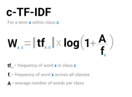
1. It applies the ctfidf equation (Figure 3) to each word in each superdocument, and plonks the output into the corresponding matrix cell. This has the effect of weighting each word according to its occurrence within a superdocument, and within the corpus. The intuition is that the importance of a word is relative to its frequency within a superdocument, and inversely relative to its frequency in the corpus.

2. It normalizes each term’s term frequency in each superdocument to between 0 – 1 so that every term in every superdocument, regardless of length, is comparable. Ctfidf is L1-normalized (Manhattan) instead of L2-normalized (Euclidean), as is usual in text processing. We’ll dig into details of normalization in the VSM post, and why L1 is used instead of L2. In simple terms, this is because we are more interested in the density of terms within a superdocument cluster than in comparing distances between superdocument clusters.

At this point in the BERTopic pipeline, we have 2 outputs:-

1. The generated embeddings, which for now are laid aside, because BERTopic has switched attention to the clusters discovered by HDBSCAN.
2. The merged clusters, which are now sitting inside the DTM (or rather, Cluster-Term Matrix, since rows are superdocument clusters). To all intents and practical purposes, these are our discovered topics. BERTopic automatically applies topic labels to these clusters using the top 3 most important words for the clusters.

There is a final, optional step to finetune the discovered topics. The BERTopic site has several tips and suggestions on how we can finetune topics, and in fact, we have experimented with that in our Jupyter notebook.

This concludes Part 1 of this post. In Part 2, we’ll have a look at our PubMed abstracts exercise.