
Imagine a vast library where every book, sentence, and word needs a shelf address — but instead of a Dewey decimal number, each piece of text gets a list of, say, 768 numbers that acts like GPS coordinates in a huge conceptual space. Things that mean similar things end up near each other in that space; things that mean different things end up far apart. A text embedding is the process of drawing that map and reading off the coordinates.
Granularity is the question of what you’re giving coordinates to — a single word, a whole sentence, or an entire document.
Context is whether a word gets the same coordinates every time it appears (so “bank” always maps to the same spot) or whether its coordinates shift depending on the words around it (so “bank” near “river” lands somewhere different from “bank” near “loan”).
Target is what the map was drawn to capture — some maps are built so that synonyms cluster together; others so that words appearing in similar sentence positions cluster together. The choice of training objective governs target: a model trained on semantic similarity tasks encodes topical and paraphrase meaning; one trained on next-token prediction encodes syntax and positional structure; one trained on knowledge-graph triples encodes relational facts.
Formally:
A text embedding is a function f that maps a discrete linguistic unit — at any level of granularity (character, subword, word, sentence, or document) — to a dense, real-valued vector in ℝⁿ, such that geometric relationships in that space reflect meaningful linguistic properties.
Another analogy I used in a previous post is that of a misshapen multi-colored stuffed toy, which you stuff into a box. The toy is still there, but it’s now a compact cube, with all the colors now concentrated. Yet another metaphor could be zip files. You zip files so that they occupy less disk space, so you also zip documents into dense embeddings. The difference is, to make use of zip files, you’ll have to extract the contents, whereas for embeddings, you use them as-is, no unzipping needed.
Text embeddings are essentially an extension of the vector space model (VSM), and you visualize them as an embedding matrix. Here is a toy example of an embedding matrix based on word granularity. If it looks vaguely familiar, it is because it resembles its ancestor, the document-term matrix (DTM), where the rows are documents, columns are words, and cells contain either raw word counts or TF-IDF values. The rows in this example are words, and the columns are the embedding dimensions. Each cell entry reflects some value of that row’s word in its column’s dimension. These values are not interpretable to us. An embedding space is thus a type of vector space.
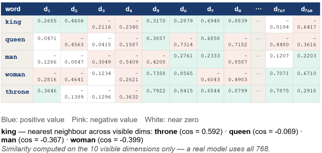
Embeddings have many advantages over plain old DTMs. For one, they are dense, and thus reduce dimensionality. Second, today’s embeddings are contextual, that is a given word can have as many embedding vectors as it has meanings, as in the classic example of money bank vs river bank. And finally, they are transferable. An embedding trained on one corpus can be ported to another.
A Brief History of Embeddings
Text embeddings did not arrive fully formed. They are the product of roughly four decades of incremental problem-solving, each generation inheriting the limitations of its predecessor and extending what was possible.
The earliest approaches represented documents as sparse, high-dimensional vectors of word counts or term frequencies. Techniques such as TF-IDF weighted terms by how distinctive they were across a corpus, and Latent Semantic Analysis applied matrix factorisation to uncover hidden topic structure. These methods were computationally tractable and well-understood, but they encoded only the surface form of text: which words appeared, not what they meant. Synonyms were invisible to them, polysemy was unresolvable, and the vectors grew with vocabulary size, triggering the curse of dimensionality.
The breakthrough came in 2013 with neural word embedding models, particularly Word2Vec and shortly after GloVe. These models trained shallow neural networks to predict words from their context (or context from words), producing compact, dense vectors in which semantic relationships were geometrically encoded for the first time. “King” and “queen” ended up near each other; arithmetic on vectors produced coherent analogies. These were stationary embeddings: every word received one fixed vector regardless of the sentence it appeared in. The word “bank” received a single vector that blended its financial and riverbank senses indiscriminately.
The next step, arriving around 2018, was context-sensitivity. Transformer-based models (most prominently BERT) processed the entire input sequence simultaneously, allowing every token’s representation to be conditioned on every other token through attention. The word “bank” in “she deposited money at the bank” now received a different vector from “bank” in “the otter climbed the steep bank.” This resolved polysemy by design. However, these contextual vectors were not immediately useful for comparing arbitrary sentences: raw BERT embeddings clustered in a narrow region of the high-dimensional space (a problem called anisotropy), making cosine similarity an unreliable measure of semantic relatedness. Fine-tuning specifically for sentence comparison (eg Sentence-BERT) corrected the geometry, producing spaces where similar sentences sat close together.
The current embedding landscape is characterised by two dominant paradigms. Contextual embeddings – transformer models fine-tuned for sentence comparison – remain widely deployed for tasks where a well-calibrated similarity space is needed. Universal embeddings extend this further: large language models fine-tuned with contrastive objectives across hundreds of tasks and dozens of languages produce a single model that can handle retrieval, classification, clustering, and semantic similarity, with the target property steered by a task instruction supplied at inference time.
The Granularity Spectrum
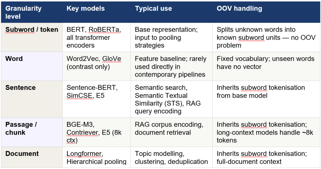
Transformer models are token-level machines at their core: they process a sequence of tokens and return one vector per token. Currently, subword tokens are the dominant granularity in language models, as they are efficient at handling out-of-vocabulary tokens. Everything coarser than a token (sentence, passage, document) requires an explicit aggregation step by the model. The differentiation among models is essentially in the output vectors – whether these represent a word, a sentence, a chunk/passage, or an entire document. The table below shows some representative models for each granularity and their typical use cases.
What Do Embeddings Encode?
Actually, embeddings can also encode images, video and audio, and much else. They aren’t mutually exclusive either – vision-language models encode both vision and text. But if you understand text embeddings, you’ll have no problem grasping other embedding types. Text embeddings can encode several aspects of text:-
- Most intuitively, they encode the semantic meaning of text, clustering similar texts together in the embedding space.
- They can also encoding position of text, that is, the position of a token in relation to other tokens in a text sequence. This, in fact, forms one of the key pillars of the attention mechanism in transformers.
- Less well known, but increasingly important in healthcare, embeddings can encode relationships among entities in a knowledge graph. These relationships are typically defined as triples (known in the jargon as RDF (Relationship Description Framework) triples) of SOURCE -> RELATIONSHIP -> DESTINATION. Graph nodes and edges also contain information that can be encoded, such as centrality, betweenness and community that can be captured into embeddings.
Evaluating Embeddings
As in other evaluations in machine learning, you can conduct intrinsic and extrinsic evaluation. Intrinsically, you would want to evaluate the embedding space’s geometry. Is it uniform (vectors are distributed evenly in the space)? Is it aligned (similar items are close together)?
Extrinsically, you would evaluate the embedding on the task(s) that the model using the embedding performs. For similarity-targeted models, does cosine similarity correlate with human similarity judgements? For retrieval-targeted models, are relevant passages found at the top of the ranked list? In such scenarios, you can’t separate out the embedding from its model, so essentially, you’re evaluating the entire pipeline.
Finally, for benchmarking, the Massive Text Embedding Benchmark (MTEB) and its successor, the Massive Multilingual Text Embedding Benchmark (MMTEB), have emerged as the definitive benchmarking tool for embeddings. The topic is broad enough to warrant another blog post by itself – I might get down to it eventually…. For now, a quick summary is that the MTEB evaluates models across 8 NLP tasks – retrieval, classification, clustering, semantic similarity, reranking, pair classification, summarization and bitext mining. The MMTEB expands this to 130 tasks in 250 languages.
(This post was written with Claude Sonnet 4.6’s help.)
Leave a Reply