In our last post, we looked at how BERTopic works. In the accompanying Jupyter notebook, we used BERTopic to extract topics from 5000 random PubMed abstracts from a dataset assembled by Huggingface user owaiskha9564. Here, we’ll run through the results, to illustrate what we can do with BERTopic.
Discovered Topics
After clustering and finetuning, the model returned 61 topics, which we used a language model (LM) optimized for clinical text, MedGemma1.5-4b, to conveniently label. Nearly all the labels made sense, except for one rather mysterious “Hemorrhage Diagnosis” for which I pulled out the representation to study further. It reads:
[(‘patients’, np.float64(0.027917486608856703)), (‘diagnosis’, np.float64(0.026417612300799875)), (‘bleeding’, np.float64(0.024901275791185475)), (‘therapy’, np.float64(0.015319996802860718)), (‘hemorrhage’, np.float64(0.015217886572923122)), (‘cranial’, np.float64(0.014582847977053592)), (‘ci’, np.float64(0.013687877858091198)), (‘cases’, np.float64(0.01330872942611377)), (‘risk’, np.float64(0.01309258588671222)), (‘case’, np.float64(0.012850121239623225))]
You can make out that it is probably about case studies of possibly intracranial hemorrhage. (‘ci’ probably means ‘confidence interval’, which we should in future remove as a stopword.)
In your actual projects, you probably want to review more rigorously the labels generated by LMs.
Finding Similar Topics
We can also look for topics that are similar to, say, “diabetes”. The numbers reflect cosine similarity. Those poor lab mice….
[(‘insulin’, np.float64(0.07505057041840049)), (‘glucose’, np.float64(0.06449658395331292)), (‘diabetic’, np.float64(0.05262164962008938)), (‘rats’, np.float64(0.046001592272389244)), (‘beta’, np.float64(0.03388939750848574)), (‘pancreas’, np.float64(0.02949886994259258)), (‘secretion’, np.float64(0.024190927374734113)), (‘diabetes’, np.float64(0.02414189329120224)), (‘mice’, np.float64(0.023805660928468596)), (‘pancreatic’, np.float64(0.022874374276756034))]
Visualizing Documents
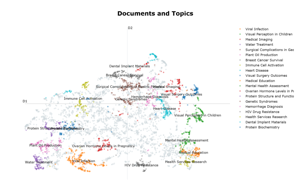
Figure 1 shows documents as points in a 2D visualization reminiscent of the Matterhorn, with the top 10 largest clusters (ie topics) highlighted in various colors. Some observations can be made about the geography of this visualization: –
- The top 10 largest clusters seem to occupy the periphery of the visualization. This is largely due to how UMAP works, because the visualization was created using UMAP. UMAP prioritizes preserving tightly cohesive groups of documents which get pulled into dense islands. Because they have strong internal connectivity and weak links to everything else, they get placed far from the center of the visualization ie peripheral position signal semantic coherence.
- By this same logic, noise in this visualization gravitates towards its center, which doesn’t look particularly sparse. This can be confusing, because intuitively, we expect noise to be found, by definition, in regions of sparsity. To reconcile this cognitive dissonance, just recall that the visualization reflects UMAP’s behavior rather than the vector space topography per se.
- Similar topics are located close to one another eg “Health Services Research” and “Medical Education”.
Keywords associated with Topics
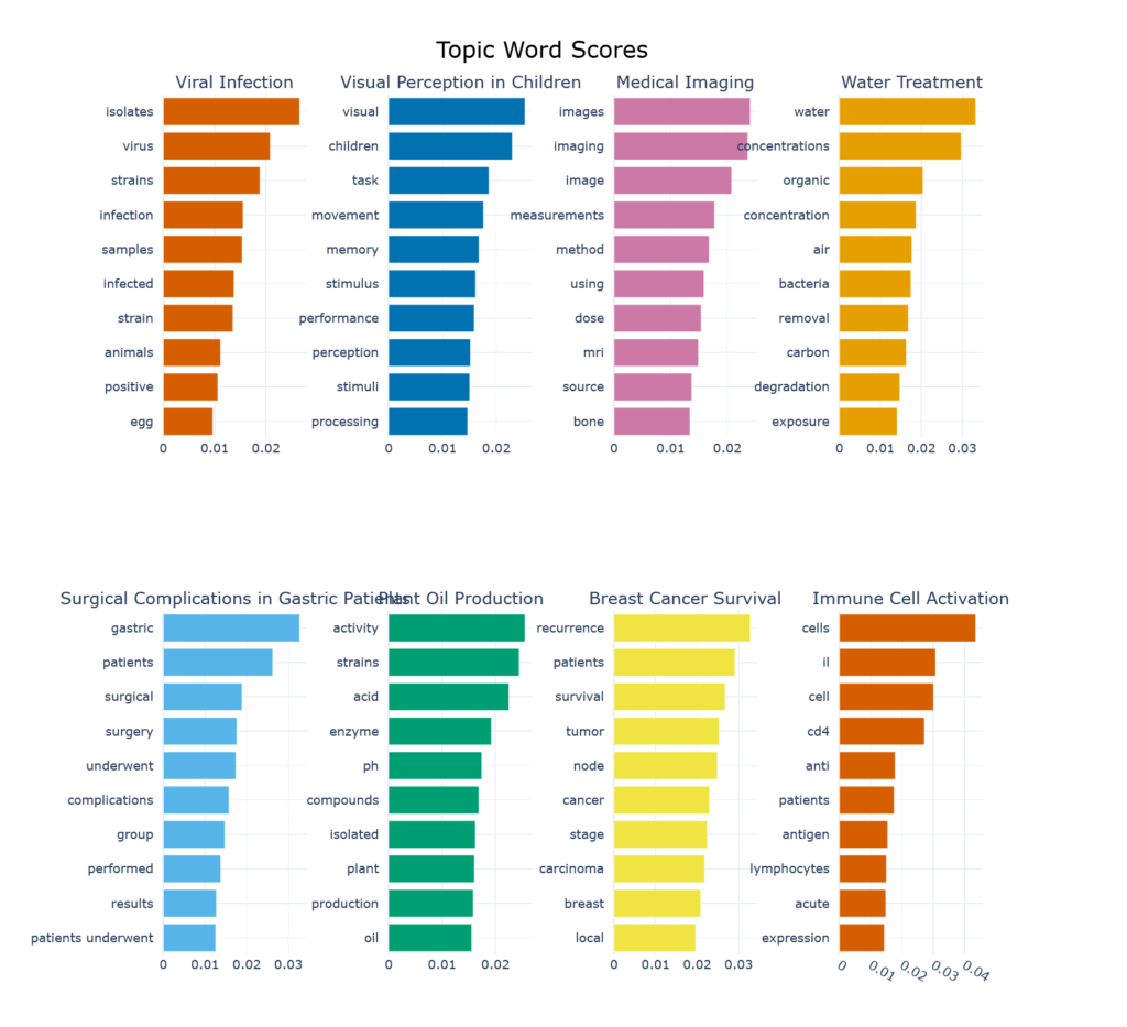
Figure 2 shows the keywords associated with the top 8 topics (so as to fit the blog page, no sinister reason) and their contribution to the topic. We can now see why “Plant Oil Production”, which evokes images of canola fields or oil palm plantations, is such a prominent topic in biomedical literature. This label might benefit from a bit of revision…
Topic Distribution of One Document
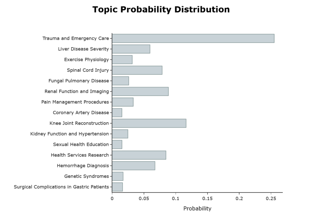
Figure 3 shows the topic distribution of the first abstract. For reference, here is the abstract: –
‘we reviewed the patterns of injuries sustained by consecutive fallers and jumpers in whom primary impact was onto the feet. the fall heights ranged from to ft. the patients sustained significant injuries. skeletal injuries were most frequent and included lower extremity fractures, four pelvic fractures, and nine spinal fractures. in two patients, paraplegia resulted. genitourinary tract injuries included bladder hematoma, renal artery transection, and renal contusion. thoracic injuries included rib fractures, pneumothorax, and hemothorax. secondary impact resulted in several craniofacial and upper extremity injuries. chronic neurologic disability and prolonged morbidity were common. one patient died; the patient who fell ft survived. after initial stabilization, survival is possible after falls or jumps from heights as great as feet it is important to recognize the skeletal and internal organs at risk from high-magnitude vertical forces.’
How HDBSCAN Works
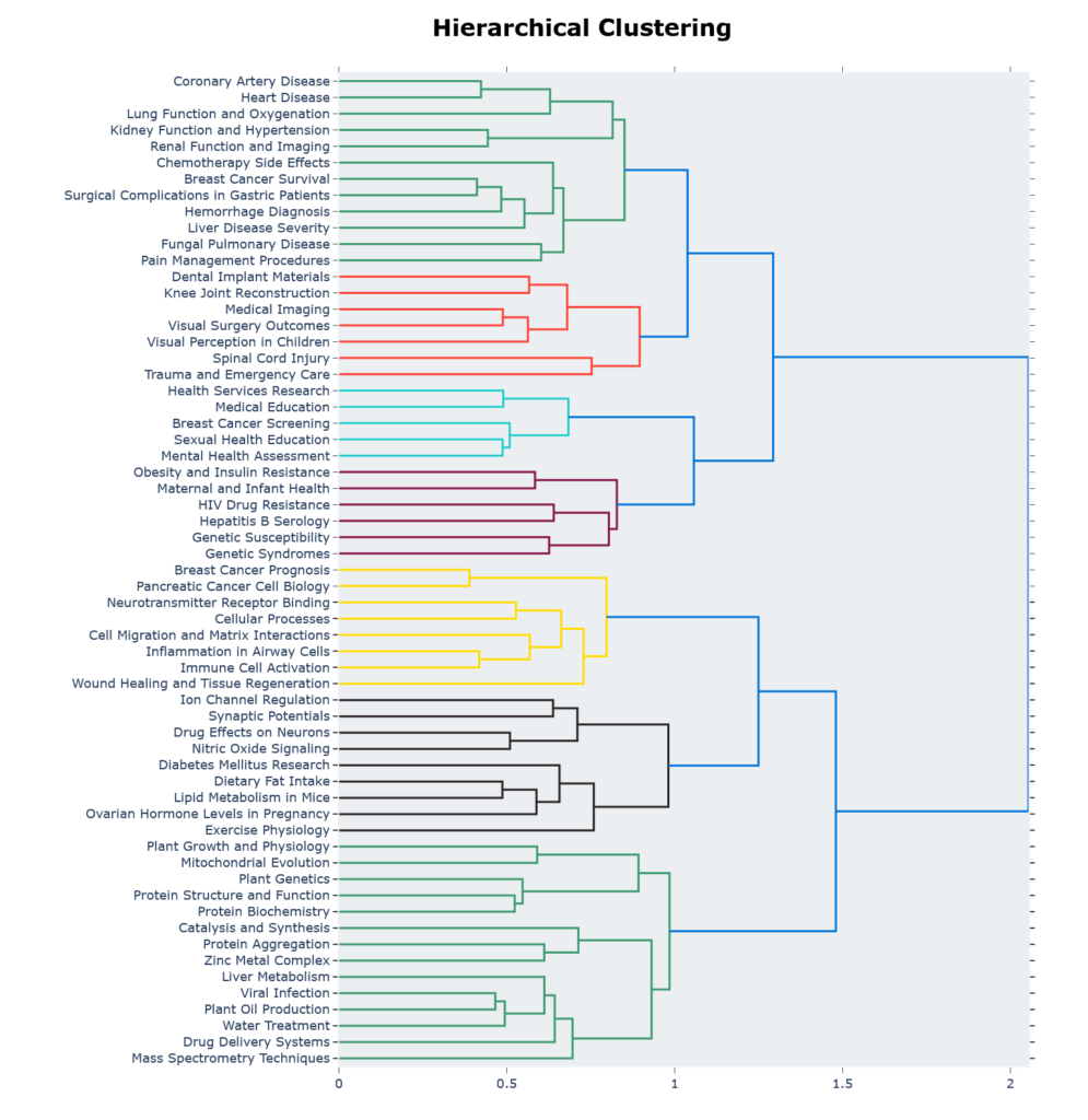
Figure 4 shows the hierarchical clustering generated by HDBSCAN.
Similarity Heatmap
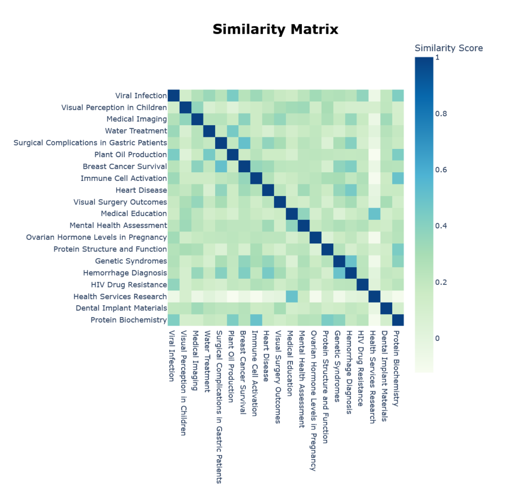
We can also see which topics are semantically close through the built-in heatmap in Figure 5.
Closing Thoughts
You may recall that in the post on Latent Dirichlet Allocation (LDA), we found that the model, at 4 topics, had the best combination of coherence (UMass = -1.96) and perplexity. At this coherence, the LDA model is actually better than BERTopic’s best of UMass = -4.5. But I would think no one imagines a PubMed dataset of 5000 abstracts can contain only 4 topics. In case you were wondering, MedGemma labelled them as ‘Gene Sequence Analysis’, ‘Clinical Trial Study’, ‘Cellular Biology’ and ‘Cancer Research’ which can serve as rather large categories, but is not going to be very useful for most practical purposes.
You might also have noticed that I did not use perplexity as an evaluation metric for BERTopic. The reason is is really quite straightforward. Perplexity is calculated from probability distributions on words, whereas in BERTopic, we’re not working with probability distributions, but clustering documents.
I thoroughly enjoyed researching for this series of posts on topic modelling, and learnt a lot in the process, and hope you’ve too.
Citation: Grootendorst M. BERTopic: Neural topic modeling with a class-based TF-IDF procedure [Internet]. arXiv; 2022 [cited 2026 Feb 15]. Available from: http://arxiv.org/abs/2203.05794
Leave a Reply